Chapter 8 Observing the extracted variables
The fused frame D is now an ordinary federated data frame, so from here we use
plain dsBaseClient. Every statistic below combines sufficient statistics from
all three sites; every plot is disclosure-controlled on the server before
anything is returned.
8.1 A derived feature: age
We turn birth_year into age as of 2020 with a single server-side expression.
ds.make() reports back that the variable was created and passes its validity
check on every site:
ds.make("(2020 - D$birth_year)", "age")
#> $is.object.created
#> [1] "A data object <age> has been created in all specified data sources"
#>
#> $validity.check
#> [1] "<age> appears valid in all sources"
We then confirm the values are sensible — on the first site, age is numeric and
its distribution sits in a plausible human range (the pooled view follows below):
ds.summary("age")[[1]]
#> $class
#> [1] "numeric"
#>
#> $length
#> [1] 889
#>
#> $`quantiles & mean`
#>       5%      10%      25%      50%      75%      90%      95%     Mean
#> 41.00000 44.00000 50.00000 59.00000 69.00000 83.00000 98.00000 61.54106
The mean age sits near 62 — older than a present-day population, but expected here. The GiBleed cohort is a frozen synthetic snapshot (Synthea-generated, released 2019-05-25, with records ending 2019-07-03), and no person in it is born after 1986. Because the data are fixed at that 2019 horizon we derive age against a constant reference year (2020) rather than the system date: a Sys.Date() value would drift on every rebuild, whereas a fixed anchor keeps the figures in this chapter reproducible.
8.2 Prevalence over the full cohort
Because absent events were zero-filled (Chapter 7), these prevalences are over the whole 2 694-person cohort, not just the persons who happen to appear in a given event table. The outcome, gastrointestinal haemorrhage, affects 479 persons:
ds.table("D$gi_bleed")$output.list$TABLES.COMBINED_all.sources_counts
#>
#>  Data in all studies were valid
#>
#> Study 1 :  No errors reported from this study
#> Study 2 :  No errors reported from this study
#> Study 3 :  No errors reported from this study
#> D$gi_bleed
#>    0    1   NA
#> 2215  479    0
Its antecedent, peptic ulcer, is more common (802 persons):
ds.table("D$peptic_ulcer")$output.list$TABLES.COMBINED_all.sources_counts
#>
#>  Data in all studies were valid
#>
#> Study 1 :  No errors reported from this study
#> Study 2 :  No errors reported from this study
#> Study 3 :  No errors reported from this study
#> D$peptic_ulcer
#>    0    1   NA
#> 1892  802    0
Diclofenac exposure covers 850 persons:
ds.table("D$diclofenac")$output.list$TABLES.COMBINED_all.sources_counts
#>
#>  Data in all studies were valid
#>
#> Study 1 :  No errors reported from this study
#> Study 2 :  No errors reported from this study
#> Study 3 :  No errors reported from this study
#> D$diclofenac
#>    0    1   NA
#> 1844  850    0
8.2.1 A finding hiding in the data
The “any NSAID” flag tells us something about how the cohort was built — every single person has at least one NSAID record:
ds.table("D$nsaid")$output.list$TABLES.COMBINED_all.sources_counts
#>
#>  Data in all studies were valid
#>
#> Study 1 :  No errors reported from this study
#> Study 2 :  No errors reported from this study
#> Study 3 :  No errors reported from this study
#> D$nsaid
#>    1   NA
#> 2694    0
The flag is universal (2 694 / 2 694), so it carries no information for
a model — it is collinear with the intercept. This is why we also extracted
nsaid_n (how many NSAID records) and diclofenac (a specific agent): within
a uniformly-exposed cohort, the burden and the choice of drug are what can
still discriminate. Extracting all three let the data reveal this; we now model
the informative ones.
8.3 Pooled summaries of the continuous features
ds.mean("age", type = "combine")$Global.Mean
#>                 EstimatedMean Nmissing Nvalid Ntotal
#> studiesCombined      61.93356        0   2694   2694
ds.mean("D$nsaid_n", type = "combine")$Global.Mean
#>                 EstimatedMean Nmissing Nvalid Ntotal
#> studiesCombined      3.711952        0   2694   2694
The pooled quantiles of age:
8.4 Federated plots
A pooled histogram of age across the three sites — drawn from server-side binned counts, never individual rows:
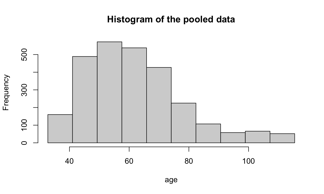
#> $breaks
#>  [1]  32.75227  41.02255  49.29283  57.56311  65.83340  74.10368  82.37396  90.64424
#>  [9]  98.91453 107.18481 115.45509
#>
#> $counts
#>  [1] 160 489 572 538 427 225 107  58  66  52
#>
#> $density
#>  [1] 0.007175728 0.021962067 0.025722805 0.024126709 0.019160386 0.010084822 0.004811924
#>  [8] 0.002599475 0.002947306 0.002323629
#>
#> $mids
#>  [1]  36.88741  45.15769  53.42797  61.69825  69.96854  78.23882  86.50910  94.77939
#>  [9] 103.04967 111.31995
#>
#> $xname
#> [1] "xvect"
#>
#> $equidist
#> [1] TRUE
#>
#> $intensities
#>  [1] 0.007175728 0.021962067 0.025722805 0.024126709 0.019160386 0.010084822 0.004811924
#>  [8] 0.002599475 0.002947306 0.002323629
#>
#> attr(,"class")
#> [1] "histogram"
And the distribution of NSAID burden (nsaid_n) — right-skewed, as drug-record
counts usually are:
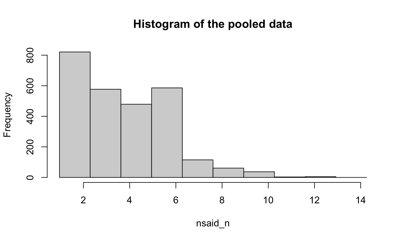
#> $breaks
#>  [1]  0.9633019  2.2922630  3.6212240  4.9501851  6.2791462  7.6081072  8.9370683
#>  [8] 10.2660294 11.5949904 12.9239515 14.2529125
#>
#> $counts
#>  [1] 821 577 479 586 115  61  37   3   5   0
#>
#> $density
#>  [1] 0.2295733933 0.1612422815 0.1336921213 0.1637645190 0.0320458351 0.0168828605
#>  [7] 0.0102698832 0.0008464201 0.0013528722 0.0000000000
#>
#> $mids
#>  [1]  1.627782  2.956744  4.285705  5.614666  6.943627  8.272588  9.601549 10.930510
#>  [9] 12.259471 13.588432
#>
#> $xname
#> [1] "xvect"
#>
#> $equidist
#> [1] TRUE
#>
#> $intensities
#>  [1] 0.2295733933 0.1612422815 0.1336921213 0.1637645190 0.0320458351 0.0168828605
#>  [7] 0.0102698832 0.0008464201 0.0013528722 0.0000000000
#>
#> attr(,"class")
#> [1] "histogram"
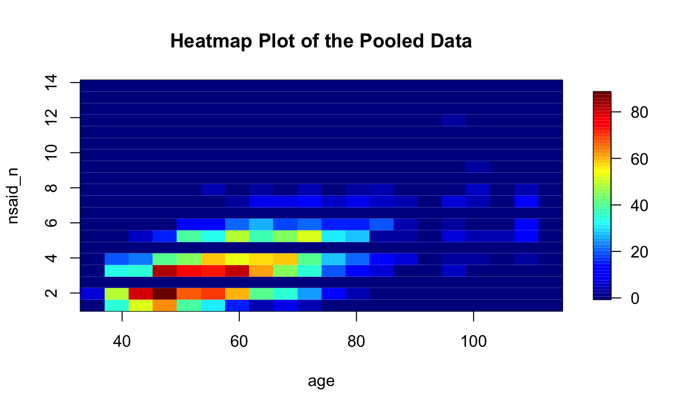
A federated heatmap shows the joint density of age and NSAID burden, with the server applying its own anonymisation to the binned surface:
8.5 The key association, previewed
Cross-tabulating the outcome against its antecedent already hints at the result the model will quantify — GI haemorrhage is markedly more frequent among persons with a peptic-ulcer history:
ds.table("D$gi_bleed", "D$peptic_ulcer")$output.list$TABLES.COMBINED_all.sources_counts
#>
#>  Data in all studies were valid
#>
#> Study 1 :  No errors reported from this study
#> Study 2 :  No errors reported from this study
#> Study 3 :  No errors reported from this study
#>           D$peptic_ulcer
#> D$gi_bleed    0   1 NA
#>         0  1679 536  0
#>         1   213 266  0
#>         NA    0   0  0
The final chapter turns this into a federated logistic regression.